Launching the GUI

Launch the graphical interface by double-clicking the SynapSpec application icon:

• Linux: Double-click SynapSpec in Applications folder
• macOS: Double-click SynapSpec in Applications folder
• Windows: Double-click SynapSpec.exe in the installation folder

Interface Overview

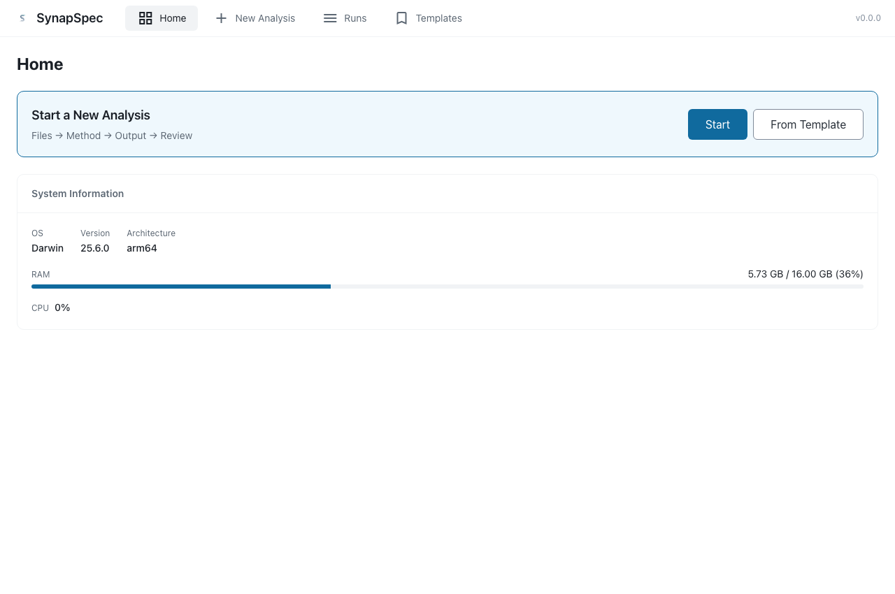
Four places, named in the header:

Section	What it is for
Home	Start an analysis, and see what the machine has to run it with
New Analysis	Set one analysis up, in four steps
Runs	What is running, what is queued, what has finished
Templates	Saved settings you can load into a new analysis

A run in progress opens on its own page from Runs. The header carries a count beside Runs when anything is queued.

New Analysis

An analysis is set up in four steps — Files, Method, Output, Review — shown as a stepper across the top. The footer moves you forward and carries the actions that apply to the whole draft: Import, Export, Reset Analysis, Save as Template.

The stepper marks what each step still needs. A step you have visited and finished wears a green tick; one you have visited and left incomplete turns red. A step you have not reached yet is just its number, in grey — an unvisited step is not one you failed to finish. Review is never marked: it requires nothing of its own, being a reading of the three steps before it.

Clicking a mark takes you to that step.

Step 1 — Files

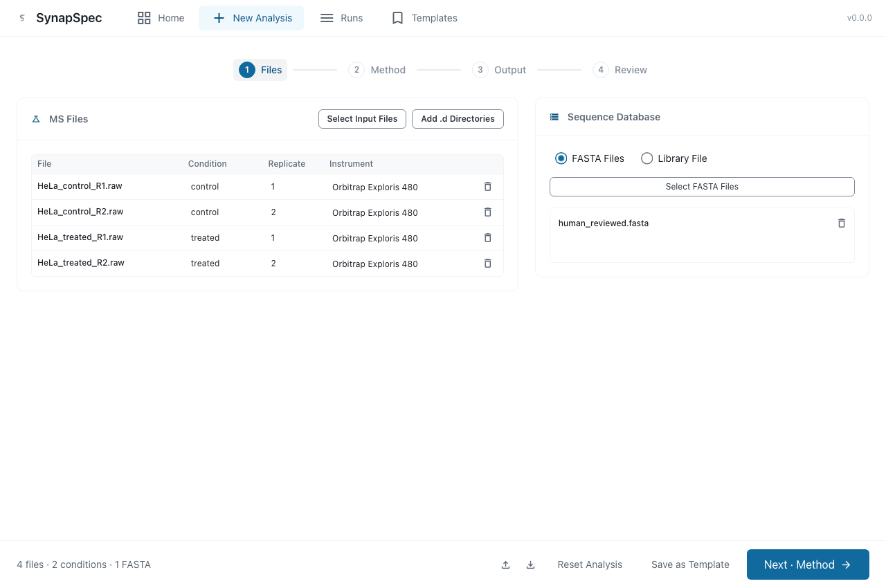
MS Files. Click Select Input Files and choose your mass spectrometry data (.raw or .mzML). Each file becomes a row where you enter its Condition and Replicate, and where SynapSpec shows the Instrument it detected from the file. Bruker .d data is a directory rather than a file, so it has its own button, Add .d Directories.

Sequence Database. Choose one of the two:

• FASTA Files — a protein sequence database search
• Library File — a spectral library search (.tsv or .txt)

The two are exclusive; picking one replaces the file list beside it.

Sample metadata for differential analysis

Differential analysis uses the metadata entered for each MS file:

• Condition: the experimental group, such as control or treated.
• Replicate: the biological replicate number. Use a positive whole number such as 1, 2, 3.

Technical runs from the same biological replicate should carry the same condition and replicate number. Before running differential analysis, fill metadata for every file, use at least two conditions with at least two biological replicates each, and make sure every input file has a unique filename.

Step 2 — Method

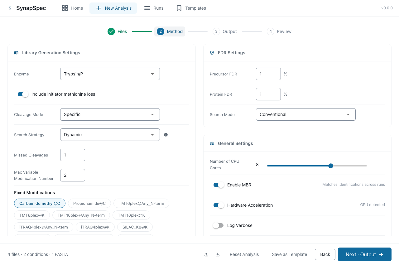
Three groups:

Library Generation Settings — enzyme, cleavage mode, search strategy, missed cleavages, the modification chips, precursor length and charge ranges, fragment types.

Both ranges are two boxes, a low and a high. Precursor Length Range is the shortest and the longest peptide; Precursor Charge Range is the lowest and the highest charge state.

Setting	Description
Include initiator methionine loss	Also generate peptides after N-terminal initiator methionine removal. On by default.

FDR Settings — precursor and protein FDR thresholds, and the Search Mode that switches between conventional and glycoproteomic analysis.

General Settings — CPU cores, MBR, hardware acceleration, and logging. Hardware acceleration is disabled when the machine has no supported device, and says so beside the switch.

Step 3 — Output

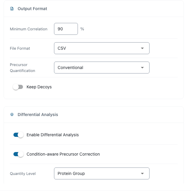
Output Directory — click Select Folder to choose where results are written.

Queue item name — the name this analysis carries in the Runs list. It is filled in for you from the file count and the date.

Output Format — minimum correlation, file format (.csv, .tsv, .parquet), precursor quantification method, and whether to keep decoys.

Differential Analysis

Setting	Description
Enable Differential Analysis	Performs pairwise comparisons between the conditions defined in step 1.
Condition-aware Precursor Correction	Refines precursor MS2 quantities within each condition using protein-level information, giving better quantities for differential analysis.
Quantity Level	The level used for the comparison: Protein Group, Precursor, or Peptide. Protein Group is the default.

When differential analysis is enabled, SynapSpec models biological replicates, combines technical runs belonging to the same replicate, and produces pairwise contrast statistics with report-ready quantity matrices.

Step 4 — Review

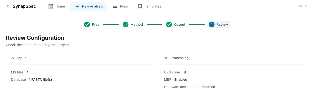
Everything the analysis will run with, on one screen: input, processing, FDR, and output. Warnings appear here — an output directory that already holds results, for instance.

Two ways to leave this step:

• Run Now — start immediately.
• Add to Queue — put it in line and set up the next one.

While an analysis is running, Run Now is refused: one analysis at a time. Everything else stays open. Build the next one, clone a finished run, load a template, and add as many as you like to the queue — that is what the queue is for.

Runs

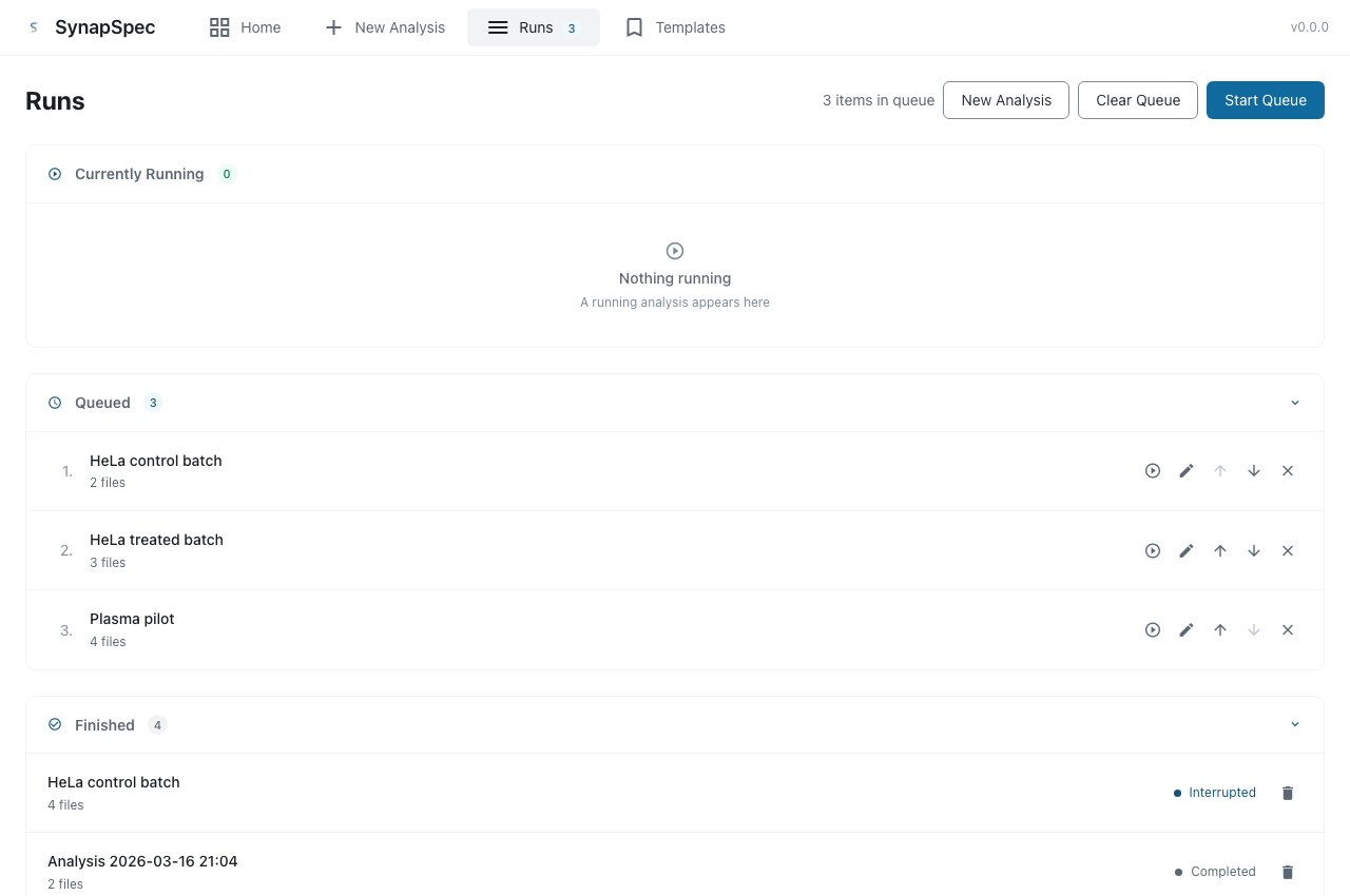
One page for every analysis, in three sections.

Currently Running — the analysis in flight. It reports the stage the engine has reached, how long it has been going, and how recently the engine last spoke.

Queued — what will run next, in order. Rows can be reordered with the arrows, edited with the pencil, or removed. Start Queue runs them one after another with no further attention; Clear Queue empties the list.

Finished — completed, cancelled, interrupted and failed runs, each with its status.

A finished run

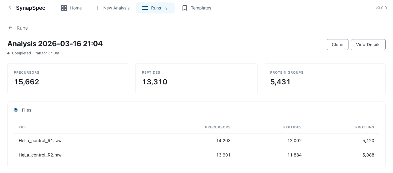
Selecting a run opens its own page. It reports what the run identified — precursors, peptides and protein groups — and the same three counts for each raw file, read from the tables the analysis wrote. Below that are the settings it ran with, the output directory, and the log.

Clone starts a new analysis from this run’s configuration: the wizard opens on step 1 with its files, database and settings already filled in, ready to change whatever you want to vary.

A run still going shows its stage and progress in the same place; the counts appear when the analysis has written its tables.

Templates

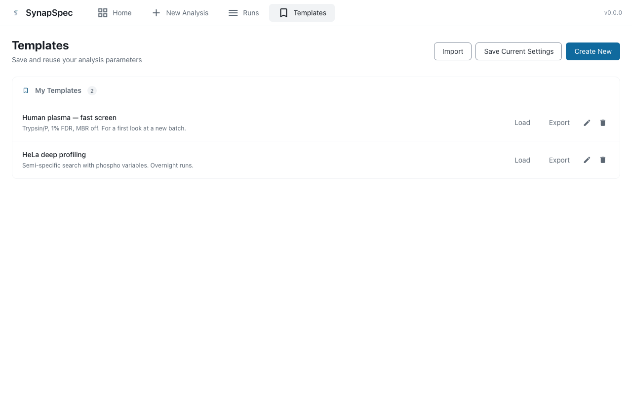
A template is a saved set of analysis settings without the files. Load puts one into a new analysis; Export writes it to disk and Import reads one back, which is how a template moves between machines.

Two buttons make a template, and they are not the same. Save Current Settings keeps the settings you have configured under a name you type. Create New opens the full editor, seeded from those same settings, for writing a template on purpose.

The New Analysis footer has the first of these too, as Save as Template.

Glycoproteomic Analysis

SynapSpec identifies N-glycopeptides through the Search Mode setting in step 2, Method.

Mode	Description
Conventional	Standard proteomics search (default)
Glyco Proteomics	Enables N-glycopeptide identification

Note: Only N-glycosylation is supported. O-glyco and other glycan types are not available.

Selecting Glyco Proteomics reveals an N-Glyco Configuration panel with two settings.

Allowed Precursor Charges — the charge states considered during glycopeptide identification. It is a row of the numbers 1 to 10 rather than two boxes: click one end of the span you want, then the other, and every number between them lights up. Nothing changes until the second click. Click the same number twice for a span of one. The default is 3 to 7. Glycopeptides carry higher charge states than ordinary peptides because they are larger; widen or narrow the range to match your experiment.

Max Missed Cleavages — the maximum number of missed tryptic cleavage sites allowed for glycopeptide candidates. Accepts 0 or more; the default is 2. This is independent of the missed cleavages setting in Library Generation Settings, which applies to the conventional search only.

Output Results

After the analysis completes, SynapSpec writes its result files to the output directory you chose. See Output Files for what each one contains.